
Quantum Quest: An RPG Tale of Superposition and Entanglement
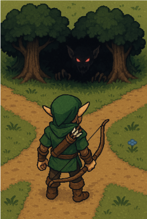
Imagine you’re playing an RPG. Your character, let’s name him Nuno, gets to a crossroads, and you have two possible roads to follow: path…

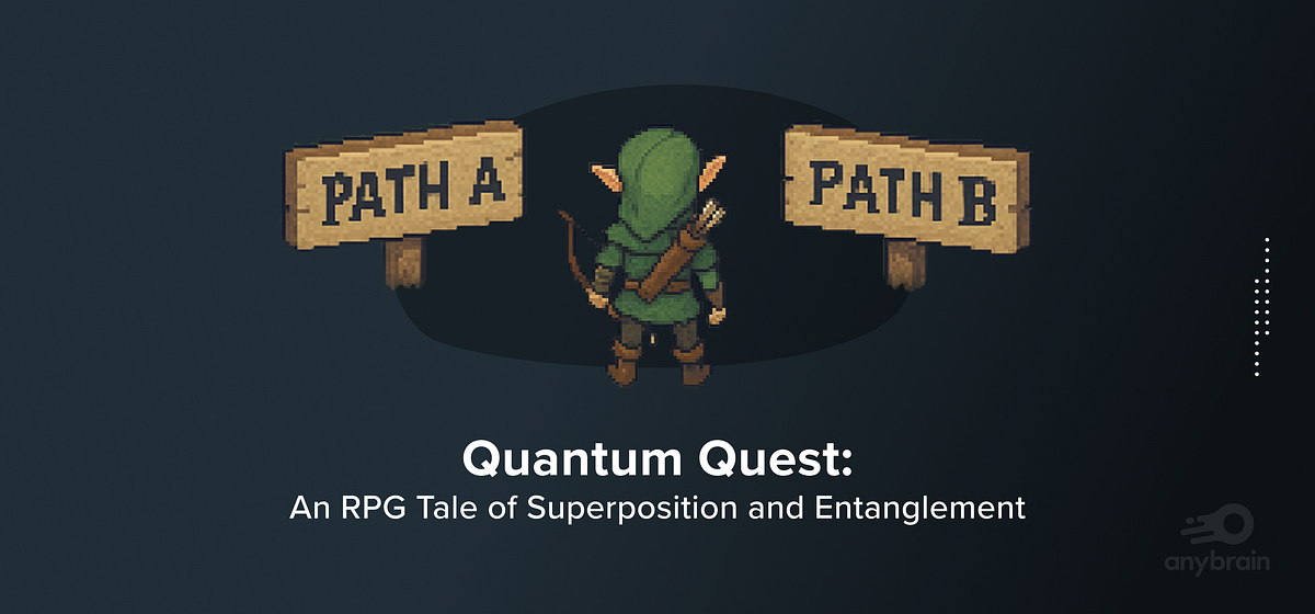
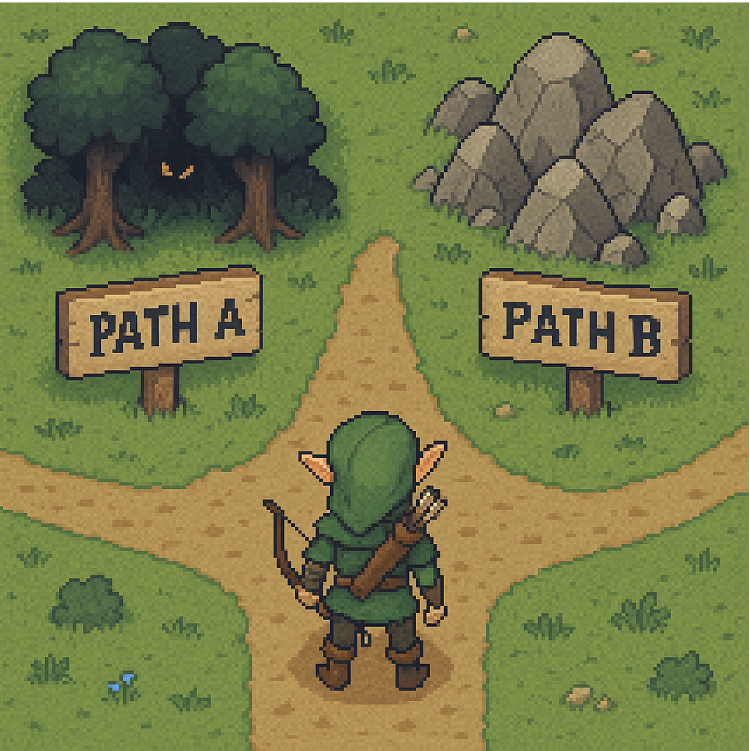
Imagine you’re playing an RPG. Your character, let’s name him Nuno, gets to a crossroads, and you have two possible roads to follow: path A, a dark forest or path B, a rocky mountain. You can only choose one, but you can explore each path before deciding. In classical computing, Nuno can only explore one path at a time. You could start by exploring path A first, gathering data, bosses fought, loot found, traps fallen, and return. Then you explore path B, gather more data, and compare. This works, but exploring one at a time is time-consuming, and resources are limited! And now imagine if it were 100 different paths, exploring each one sequentially would be a serious grind.
But, what if we are not in a classical environment? What if your character has a special ability called superposition, which allows them to exist in multiple realities at once? Instead of exploring one path at a time, your character “splits” across all paths simultaneously. Now, with this ability, we can gather all the data we need in a fraction of the time! Also, in this version, you have a travel companion, named Carlos, and both Nuno and Carlos are linked. If Nuno finds a healing potion recipe, Carlos will also benefit from it. If Carlos falls into a trap, Nuno will adjust the course without even having to see Carlos in the trap. This is entanglement, in the state that the duo shares knowledge instantly, which improves the decision-making of the duo.
This teamwork means that they are evaluating all paths in parallel, like exploring every single quest of a storyline at the same time. This not only makes the decision process much faster but also more informed. So, now you’re at a point where Nuno’s and Carlos’ experiences interact and interfere with each other. Where successful paths, with high rewards, reinforce each other, and low-rewards or dead ends cancel each other out. In the end, when Nuno makes a final choice, it won’t be random; you won’t forget path number 75, or mix path number 2 with path number 6, all paths are weighted in this final choice, which is the most promising path.
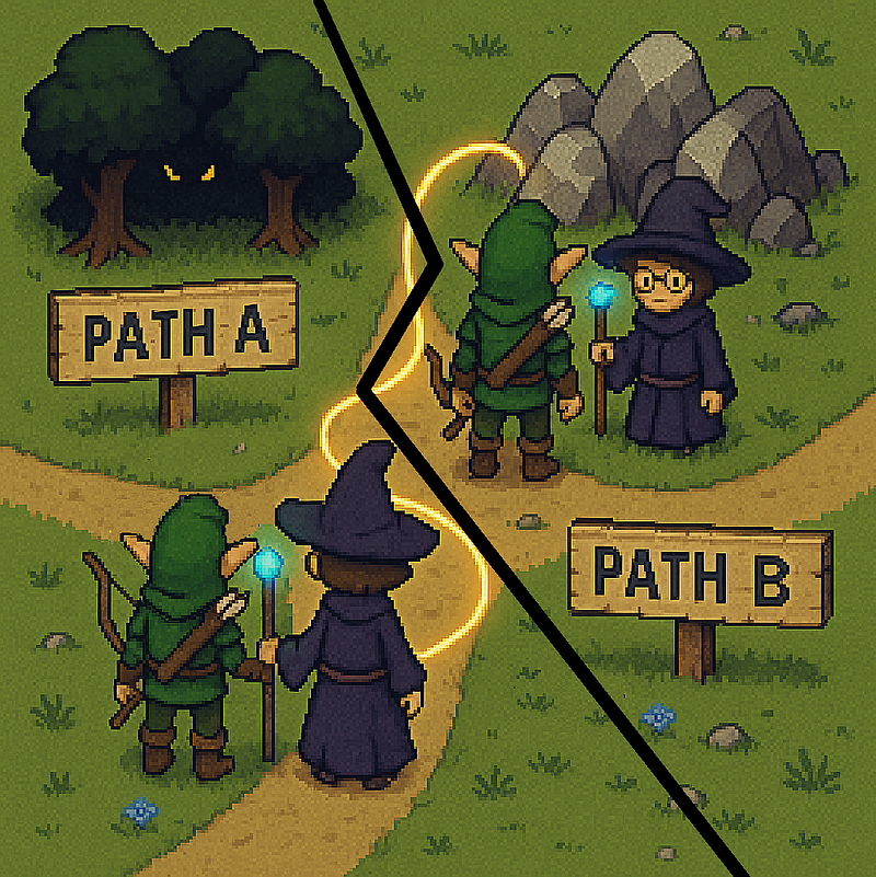
Superposition, entanglement, parallelism and interference are some of the key phenomena that make quantum computing so different from classical computing. Not only is it faster, but smarter, more optimised for decision-making and better suited to scale with increasingly complex problems, like, what if we had 1000000 paths!
Of course, these phenomena have been simplified to fit within the RPG example. In reality, they involve complex mathematics and physics, which we won’t discuss here. The objective is just to give a feel for how differently quantum computing works from classical computing.
So, how does this matter in data science? Let’s think of every decision our RPG has to make as optimising models, searching for patterns, choosing model features, and many others. We can see how beneficial quantum computing would be for data scientists, who often have to deal with massive and complex problems. And, let’s be honest, classical tools struggle with high-complexity problems. This is where quantum computing shows promise, enhancing our ‘toolbox’ for the kinds of data challenges that are becoming too big for classical methods.
Treasure Hunting with Quantum Tricks
Let’s see this advantage through a practical example, still using our gaming analogy.
Imagine we have 32 paths, and only one of them hides a treasure. The rest are empty. This is a classic search problem, and to solve it, we can take two strategies: a classical brute force search, or a quantum search, using Grover’s Algorithm.
The classical Brute Force
In the classical approach, we search each path one at a time. In the worst-case scenario, there’s a possibility that we have to search all paths. This means we might have to check all 32 paths to find the path we want. So, for N possible paths, this strategy takes O(N) time.
Quantum Grover’s Algorithm
On the other hand, Grover’s algorithm can find the correct path in only √N steps! For 32 paths, this is about ~6 steps. Therefore, for N possible paths, it would only take O(√N).
To better understand the logic behind Grover’s search, let’s simplify the problem: suppose we know the exact path code we’re looking for, we just need to search for it within a list of possible paths? Imagine each path name is defined as a unique combination of 1’s and 0’s, like ‘01001’ — in quantum computing, such binary strings correspond to quantum states, represented in Dirac notation, just like |01001⟩.
For the brute-force approach, it is very straightforward, as the name suggests. We check each path; if it is what we want, it stops!
But, for Grover’s algorithm, it is not that simple. Remember reading about superposition, interference and entanglement in the intro? Well, that is what makes it fundamentally quantum!
We start with creating a superposition of all possible states, which means the quantum system is in a mix of all N paths at once (something only quantum computers can really do).
In the next step, we create a function called oracle, which is a quantum function that marks the path we want by flipping the sign of the state (our path name). For example, in classical terms, it’s like a function f(x) that returns 1 if x is what we are looking for, and 0 if otherwise. In the quantum version, we have:
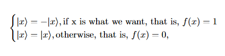
This function sets up interference for the next phase, called the diffuser. In this step, it uses interference to amplify the probability of the states that correspond to the wanted solution, and fades the ones that do not.
It then proceeds to repeat the previous steps, for about N times. By repeating, it increases the probability of the correct path. Finally, the quantum system is measured, and it returns the solution state, with a high probability of being the path we were looking for!
from qiskit import QuantumCircuit, transpile
from qiskit_aer import Aer
from math import floor, pi, sqrt
import time
import matplotlib.pyplot as plt

def diffuser(n):
  # This function creates a diffuser gate for Grover's algorithm
  # This gate boosts the probability of measuring the correct path

  diff = QuantumCircuit(n) # Create a quantum circuit with n qubits
  # Perform some quantum gate actions that make up the diffuser
  diff.h(range(n))
  diff.x(range(n))
  diff.h(n-1)
  diff.mcx(list(range(n-1)), n-1)
  diff.h(n-1)
  diff.x(range(n))
  diff.h(range(n))
return diff

def phase_oracle(n, target_index):
  # This function creates the oracle, the gate that marks the correct answer
  # It flips the sign(phase) of the target state
  # The marking helps the diffuser know which answer to amplify.

  oracle = QuantumCircuit(n)
  binary = format(target_index, f'0{n}b') # Converts the target to binary (e.g., '111')
  for i, bit in enumerate(binary):
    if bit == '0':
      oracle.x(i) # Apply a flip
  oracle.mcx(list(range(n-1)), n-1) # Marks the target
  for i, bit in enumerate(binary):
    if bit == '0':
      oracle.x(i) # Undo the flips
return oracle

max_qubits = 20 # Set maximum number of qubits, in this case to run the Grover's algorithm for 2 to 20 qubits (search space)
backend = Aer.get_backend('qasm_simulator') # Get a virtual quantum computer (a simulator)
brute_steps = [] # Array to save the number of steps with the brute force approach
grover_steps = [] # Array to save the number of steps with Grover's algorithm
simulation_times = [] # Array to save how long the quantum simulation took

# For each number of qubits from 2 to max:
for n in range(2, max_qubits + 1):
  N = 2**n # Total number of possible paths
  target = N - 1 # Set the target as the last item ( to test the worst case scenario)
  num_iterations = floor((pi / 4) * sqrt(N)) # Calculate number of Grover steps

  # Create a quantum circuit
  qc = QuantumCircuit(n)
  qc.h(range(n)) # Initialise in superposition (put the system into a state of equal possibility)

  oracle = phase_oracle(n, target) # The gate that marks the correct answer
  diff = diffuser(n) # The gate that amplifies it

  # Repeat the process
  for _ in range(num_iterations):
    qc.append(oracle.to_gate(), range(n))
    qc.append(diff.to_gate(), range(n))
  qc.measure_all() # Measure the result

  # Simulate and time how long it takes
  start = time.time()
  compiled = transpile(qc, backend)
  result = backend.run(compiled, shots=1024).result()
  end = time.time()

  counts = result.get_counts() # Count how often each answer came up
  simulation_times.append(end - start)
  brute_steps.append(N)
  grover_steps.append(num_iterations)

# Draw a graph showing how many steps each method took
plt.figure(figsize=(12, 6))
plt.plot(range(2, max_qubits+1), brute_steps, label="Brute-force steps (O(N))", marker='o')
plt.plot(range(2, max_qubits+1), grover_steps, label="Grover steps (O(√N))", marker='s')
plt.xlabel("Number of Qubits")
plt.ylabel("Steps")
plt.legend()
plt.grid(True)
plt.tight_layout()
plt.show()
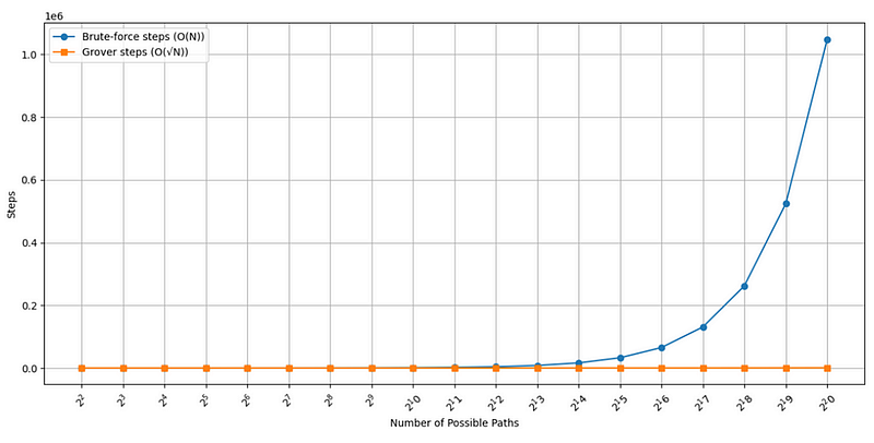
We’ve seen the basic idea behind Grover’s algorithm, but how does it perform as the number of paths grows?
Let’s look at the performance difference between the classical and quantum approaches mentioned above. In the plot below, we compare the number of steps each method takes as the number of ‘paths’ increases.
The blue line represents the brute-force performance, and the orange line represents the Grover’s algorithm performance. The blue line grows exponentially with the number of paths; on the other hand, the orange line grows much more slowly! At 220 paths, the brute-force needs over 1 million steps, as for Grover’s algorithm only needed about 1000 steps.
Quantum Advantage: What’s Real, What’s Next?
This is one of the examples where we can see the quantum advantage in action! Other algorithms play the same advantage, in different fields. For example, in cryptography and data security, we have Shor’s algorithm that can factor large numbers exponentially faster than popular classical algorithms.
And what about data science? Quantum computing holds a promising future here! Many problems in data science involve dealing with big datasets, finding patterns in high-dimensional spaces, and optimising models. All of these are tasks where we can see that quantum algorithms could provide an edge.
Not only can quantum computers process big amounts of data much faster than classical computers, but we also have Quantum Machine Learning algorithms, like Quantum Principal Component Analysis and Quantum Neural Networks. We also have Quantum Optimisation Algorithms that are used to solve optimisation problems, etc.
Even though we are in early stages, we can see the potential!
Of course, all of this comes with challenges. One of the biggest challenges is hardware. Current quantum computers are still limited and prone to errors, which restricts the complexity of problems they can process.
We do have advanced quantum computers developed or being developed by IBM, Google, among others. For example, IBM Quantum Eagle has 127 qubits — fundamental units of quantum information, similar to classical bits but with a very different behaviour. These qubits are extremely fragile and easily disrupted by external factors and other quantum phenomena, causing errors to accumulate during computation.
And while 127 bits may sound impressive, it is still quite limited for most quantum algorithms! To outperform classical systems on meaningful problems, we would likely need thousands to millions of qubits.
Beyond hardware, there’s also the challenge of developing the algorithms. Many quantum algorithms still remain on a theoretical basis. Developing them is non-trivial: it requires new ways of thinking about problems, new mathematical tools, and a whole new, unfamiliar logic!
In addition, quantum algorithms don’t always perform better than classical ones. They often only show an advantage when the data is very large and complex — that’s where they really shine — something current systems can’t fully support yet.
Finally, there’s a resource gap. Only a small group of researchers has access to actual quantum machines. Most people rely on simulators, which don’t reflect the full potential of a quantum computer.
A Final Challenge for the Reader
We’ve seen how quantum computing opens up a world of new computational possibilities. Now, let’s take a moment and imagine this in a gaming context.
- What happens when cheat developers have access to quantum-powered tools?
- What if they create a cheat software that could simulate thousands of gameplay outcomes in parallel, and could adapt in real-time?
- Could quantum machine learning help mimic human behaviour better than ever before?
Could this even become reality? This may be thinking too much ahead, but we need to stay ahead of the curve; the race is on! So we leave you with this challenge:
How would you use quantum principles to generate the next generation of cheating software?
Bibliography
Nielsen, M. A., & Chuang, I. L. (2010). Quantum Computation and Quantum Information: 10th Anniversary Edition. Cambridge University Press.
IBM Quantum. IBM Quantum Experience. Retrieved from https://quantum-computing.ibm.com
Qiskit Textbook. Grover’s Algorithm. Qiskit by IBM. Retrieved from https://qiskit.org/textbook/ch-algorithms/grover.html
Preskill, J. (2018). Quantum Computing in the NISQ era and beyond. Quantum, 2, 79. https://doi.org/10.22331/q-2018-08-06-79
Montanaro, A. (2016). Quantum algorithms: an overview. NPJ Quantum Information, 2, 15023. https://doi.org/10.1038/npjqi.2015.23