Dealing with False Positives

The False Positive Trap

Intro

False positives matter more than most people think. In a crime investigation, accusing an innocent person can be just as damaging as missing a guilty one. A false accusation destroys trust, damages credibility, and can permanently affect the victim. The goal is not simply to catch offenders; it’s to catch only offenders.

Section 1: The Crime Scene Is Messy

If you walk into a crime scene and expect a clean trail of clues, you’ve already failed as an investigator. Real-world data is noisy and context-dependent. To build a solid case, we must first curate our evidence.

1.1 Are the witnesses reliable?

Let’s say that your labels are our witnesses. If the labels point at innocent people and swear they’re the culprit, then your model learns that ‘innocent’ looks like ‘guilty’. False positives start here!

But the opposite is just as dangerous: if real culprits are slipping into your “innocent” pile undetected, your model’s boundary becomes warped in the other direction. It learns to accept bad behaviour as “normal,” leading to False Negatives, where you miss actual threats entirely.

Audit your data! Manually check a random sample. If you find a bad witness or a mislabeled suspect, kick them out of the dataset. You cannot build a fair verdict on a foundation of perjured testimony.

To illustrate this concept, imagine the following scenario: imagine your model is looking at call patterns to catch scammers.

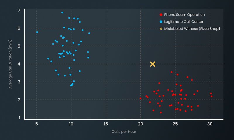
If you accidentally label a busy pizza shop as a “scammer,” the model begins to think that high call volume is a sign of guilt. It then draws a “guilty” boundary that unfairly flags every busy, legitimate business as a scam operation.

Conversely, if a real scammer hides near an incorrectly labelled “innocent” data point, the model will learn to ignore them. In short: if your training data is tainted by errors, the model will treat those mistakes as the “law,” causing it to falsely accuse the innocent and overlook the guilty.

1.2 The City Isn’t 50% Criminal

In a city of a million people, you don’t have 500,000 burglars (hopefully!). Most datasets shouldn’t be a 50/50 split between innocents and criminals in a dataset. It isn’t real, it doesn’t describe the real case scenario.

If you force a perfect balance, you create a paranoid model that arrests people for sneezing. Keep your validation data as imbalanced as the real world. Use techniques like SMOTE or Class Weights to help the model recognise rare crimes, but don’t erase the natural bias toward innocence.

1.3 Don’t Profile the Wrong Neighbourhood

If you only analyse behaviour from suburban families, you’ll probably flag night shift workers just because their schedule is different. To avoid ‘narrow data’, your training data should represent:

• different users
• different environments
• different behaviours

Because you never know where the culprit might be hiding.

1.4 Ignoring the Red Herrings

A detective shouldn’t care if a suspect is wearing a blue shirt if 98% of the city also wears blue shirts. That’s a red herring. In data, we call these unstable features. If a feature is common to everyone, like ‘uses a telephone’, it provides no insight into who is a scammer. However, do not discard noise blindly. Understanding the cause is vital, as some missing values are actually informative. Rather than deleting unstable features that fluctuate wildly, use techniques like regularisation to penalise extreme sensitivity.

Imagine you include a feature that is common to everyone, like ‘Uses a telephone’. This tells you nothing about who is a scammer.

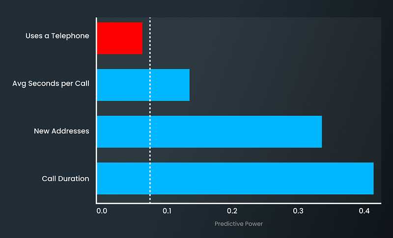
‘Uses a Telephone’ is your Red Herring. Everyone in this investigation uses a telephone! If your model spends its ‘computational budget’ trying to analyse that feature, it’s ignoring the real evidence (like New Addresses or Call Duration). It’s the data equivalent of a detective focusing on the fact that the suspect was wearing shoes. It’s technically true, but it doesn’t help you solve the crime.

Section 2: The Art of the Threshold

Setting a threshold is the moment you move from investigating to arresting. If the bar is too low, you drag innocent people to the station; too high, and the guilty walk away.

2.1 The “Heavy Tail” of Human Behaviour

While in a ‘normal’ sample, most people have a somewhat steady and predictable routine, some might be eccentric: they work weird hours or travel constantly. If you set an arrest threshold based on ‘maximum normal behaviour plus a tiny margin’, you criminalise anyone who is simply out of the ordinary.

We can visualise this idea as follows:

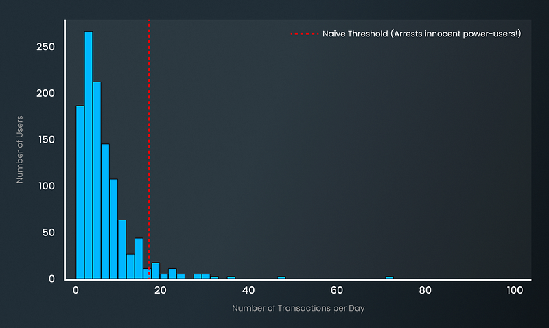
The red line is the “naive detective.” It catches the scammers, but it also drags in all those “heavy tail” innocent users who just happen to be power users. A better detective adjusts the threshold to the right, or better yet, uses individual baselines.

2.2 Dynamic Standards

You can’t apply the same standard of evidence to a part-time teenager working in a local grocery store, saving up for a PS5, as we do to a K-pop idol. A 10,000€ transfer is a major red flag for a teenager, but just a regular Tuesday for a global star.

In some cases, you might require dynamic thresholds. You should judge a suspect against his own personal ‘baseline’, not the city-wide average. If a suspect’s behaviour is 3x their own personal norm, that’s evidence; if it’s just 3x their neighbour’s, it might just be a different lifestyle.

2.3 Sequence vs Snapshot

Is a man running down the street fleeing a crime or catching a train? A single data point (a snapshot) lacks context. To get a warrant, you need the sequence. Don’t base an arrest on one event. Instead, look for the progression: (1) Loitering near property → (2) Searching for security cameras → (3) Attempting multiple entry points.

2.4 The “Multi-Clue” Requirement

In court, circumstantial evidence is rarely enough. Combine signals: Magnitude + Stability (high activity with robotic consistency) or Speed + Regularity (fast actions with perfectly uniform timing).

The figure below shows a simplified representation of this process.

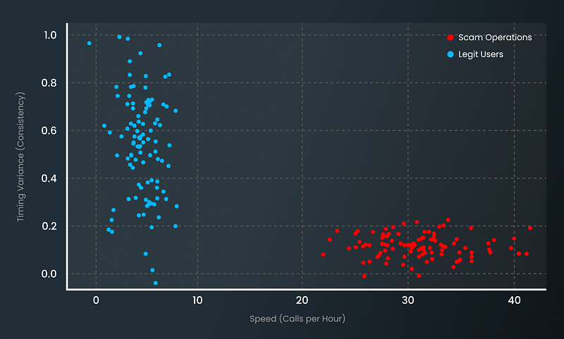
In a phone scam, a single high-value transfer isn’t enough to flag someone. If you only look at ‘Speed’, you catch some fast-talking salespeople. If you only look at ‘Consistency’, you catch some automated background tasks. But when you look at the Red Cluster (High Speed AND Low Variance), you’ve found a phone scam operation. That overlap is your ‘probable cause’.

2.5 The Detective + The Law

A machine learning model is like an informant: it’s incredibly good at spotting patterns we might miss, but it doesn’t always understand the law. A rule-based system is our ‘Law Book’, and with it, we define the non-negotiables.

Some of the strongest investigations use a hybrid system. The model flags the potential suspect, but the ‘Rules’ act as the final review before an arrest. This ensures that every flag has a logical, human-readable justification that would hold up in a courtroom.

Section 3: The Danger of “Snap Judgments”

Convicting someone based on a glance is the fastest way to ruin an investigation.

3.1 The “Non-Negotiable” Minimum

In a courtroom, if the prosecution has zero evidence, the judge dismisses the case. In your model, you need to enforce the same rule.

If a user hasn’t performed a minimum number of events or existed in the system for a minimum time window, you shouldn’t even score them. It’s better to have a ‘blind spot’ for a few hours than to flag an innocent new user as a criminal just because you lack their baseline.

3.2 The Law of Large Numbers

With few data points, the variance is steep and misleading. Plot variance against sample size. Only trust features where the variance has levelled off. This is the point where the ‘noise’ of daily life averages out.

3.3 The Smoothing Dilemma

Smoothing is like interviewing a witness three times to ensure their story is consistent. It irons out the jittery spikes that don’t really matter.

However, you have to be careful. If you smooth everything, you’ll erase the very crime you’re trying to solve.

• When to Smooth: Imagine you are monitoring the “Average Login Frequency” for an account. A user might log in 5 times one day and 15 times the next because they are busy. A single spike here isn’t a crime; it’s just life. By using a moving average (smoothing), you filter out these day-to-day jitters and establish a steady baseline. You only raise the alarm if the smoothed average remains abnormally high for an extended period.
• When NOT to Smooth: Imagine you are tracking a “System Configuration Change” event. A user suddenly disables multi-factor authentication (MFA). This is a binary, high-impact event. If you use a moving average to “smooth” this data, you might average it out with 10 previous days of “no change,” effectively muting the alert because the “average” change remains low. In this case, you do not smooth. You want to detect that single, sharp spike immediately.

Let’s see what that looks like in practice.

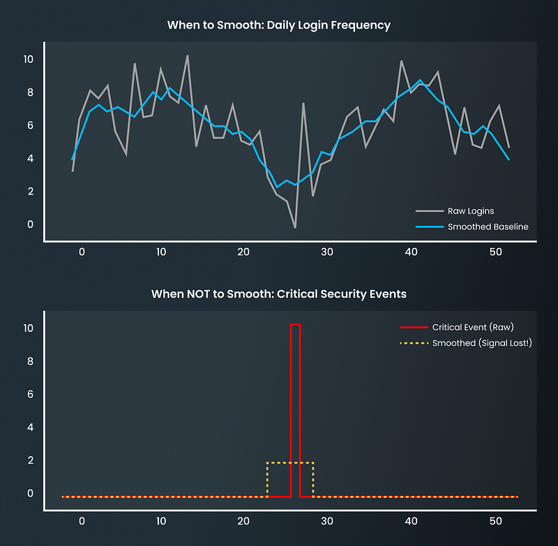
The Blue Plot: Show how smoothing is your friend when dealing with natural fluctuation. It prevents you from overreacting to a busy Tuesday.

The Red/Orange Plot: Show how smoothing is your enemy when dealing with binary threats. If you smooth the red line, the orange dashed line hides the severity of the security breach, turning a “critical emergency” into a mere “minor blip.”

Section 4: The Serial Offender

If a suspect runs through a red light, it might be an emergency or a distraction. But if they run ten red lights in a row, it’s more than that, and a high-speed chase is justifiable.

The biggest mistake a “detective” (model) can make is reacting to a single, isolated spike. Real criminal intent is rarely a momentary flash, it is a sustained pattern.

4.1 The Continuity Rule

To filter out one-off mistakes, use a continuity rule. Trigger an alarm only if you see N anomalies in a window, or if an anomaly persists for X minutes.

4.2 The Detective’s Log

In the previous chapter, we talked about smoothing data to understand a suspect. Here, we smooth the verdict to ensure we aren’t being impulsive. Think of this as the detective reviewing the entire case file before finalising the arrest report. For example, we can use:

• Sliding Window: Aggregate scores over time. If the average score crosses the threshold, the case is serious.
• EWMA (Exponentially Weighted Moving Average): This prioritises recent behaviour while keeping history in mind. It keeps you reactive to new threats while remaining steady enough to ignore random noise.

Think of it as follows:

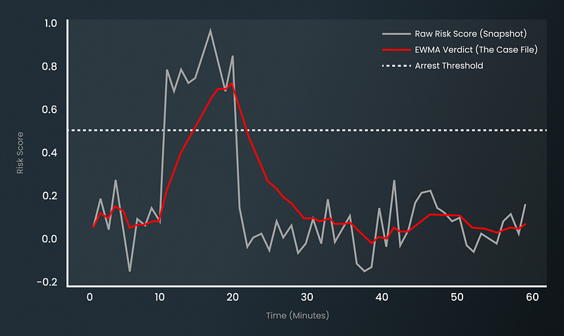
The grey line (Raw Risk Score) represents a series of individual snapshots. If you were to arrest based on this alone, you might catch a real offender, but you would also be constantly distracted by the “wobbles” of daily life.

The red line (EWMA Verdict) is your detective’s logbook. It ignores the short-lived, jagged spikes in the grey line (temporary noises). Instead, it only rises steadily when the suspicious behaviour is sustained.

When the red line finally crosses the black dashed Arrest Threshold around the 14-minute mark, it isn’t reacting to a single moment. It is proving that the suspect has been active long enough to build a clear, persistent pattern of behaviour. This is the difference between guessing and building a case: you aren’t just reacting to a bad minute; you are documenting a bad hour.

Section 5: The Contextual Jury

As mentioned before, in a courtroom, context is very important.

This is the final hurdle in reducing false positives: Context. An anomaly is just a deviation from a norm, but a crime is a deviation from the rules.

5.1 Adding Context as Evidence

By adding features like device type, environment, or platform, you turn a ‘new device’ event from a red flag into a harmless, explainable log entry.

5.2 Same Signal, Different Meaning

Identical metrics can stem from vastly different intentions. A user who performs 50 actions a minute might be a high-frequency attacker or a power user using keyboard shortcuts.

Without context, your model is forced to guess. By providing contextual metadata, you turn a vague ‘anomaly’ into an explainable behaviour profile.

5.3 Controlled Data Collection

Ensure your training set contains both ‘normal’ and ‘anomaly’ data within the same conditions. If you only show the model’s normal behaviour from public transport and ‘anomaly’ behaviour from a car, the model will mistakenly learn that cars are suspicious. You have to show both types in both contexts to force the model to learn the difference between the device and the intent.

5.4 The “Impossibility” Check

Even the best models can be fooled. This is why you must implement impossibility checks, that is, hard rules that override the model.

For example, a suspect logged in from London, then 30 seconds later from Tokyo. This is physically impossible. Combining these ‘sanity checks’ with your model creates a layered defence. If the model thinks it’s suspicious, but the impossibility rule says it’s physically impossible for the person to be the owner of the account, you have a much higher confidence level for your verdict.

Section 6: The Internal Audit

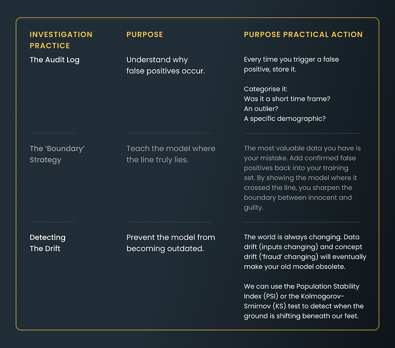
If you ignore your false positives, you are doomed to repeat them. False positives are not random accidents; they are structured patterns. If you flagged an innocent night-shift worker as a criminal just because of the schedules, they actually represent a blind spot in your ‘law’.

Section 7: Choosing Your Detective

Choosing a model is like hiring a team of investigators. You want investigators who are smart, disciplined, and don’t jump to conclusions.

7.1 Hire the Right Expert

For most anomaly detection, Random Forest, XGBoost, and LightGBM are your top candidates.

They handle non-linear relationships (the ’if-this-then-that’ scenarios) and are less sensitive to feature scaling than linear models. Models like LightGBM and XGBoost are highly efficient because they use histogram-based splitting, making them perfect for both massive datasets and smaller, niche investigations where you need a quick, reliable decision.

7.2 Don’t Let the Model Overreact

You must prevent your model from ‘memorising’ the training data (overfitting), which inevitably leads to unpredictable errors and a spike in false alerts.

To keep the model grounded, control max_depth to stop the model from building overly complex, nonsensical rules. If using gradient boosting, the learning_rate is your precision dial, so you can lower it to ensure the model learns slowly and carefully.

Use ensemble methods. Instead of relying on one ‘witness’, use Stacking or Voting to combine multiple models. When one model is ‘paranoid’, the collective ensemble averages out the bias.

7.3 Data Hygiene: The Foundation of Justice

The best model in the world will fail if you feed it biased data. Before you train, consider these practical requirements:

• Feature Quality & Outliers: While tree-based models like XGBoost and LightGBM are scale-invariant (meaning they don’t require feature normalisation), they remain highly sensitive to extreme outliers and noise. Cleaning your data isn’t about scaling ranges, but it’s about signal quality. Always scrub your features for noise and bias to ensure your “detective” is focusing on real evidence rather than anomalies in the data itself.
• Handling Missing Data: Know your tool’s relationship with NaN values. Tree-based models (XGBoost/LightGBM) are sophisticated enough to treat NaN as a meaningful category, where in many cases, the absence of data is a signal itself. This is a massive advantage over Neural Networks, which require you to manually deal with missing values.
• Managing Imbalance: Use undersampling and oversampling techniques to ensure the model respects the rare “criminal” class without hallucinating crimes in your normal population.

To illustrate this concept, imagine the following scenario:

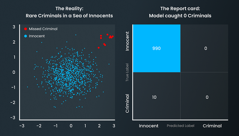
The Left Plot shows the detective the “crime scene” (99% Innocent, 1% Criminal), with the tiny red cluster being hard to find.

The Right Plot (The Confusion Matrix) is the smoking gun. Look at the bottom-right corner. It shows 0 True Positives. The model looked at 10 criminals and didn’t arrest a single one. Even though the model is technically “99% accurate,” it is 100% useless at its actual job.

Don’t let accuracy fool you. If your data is imbalanced, your model will take the easy way out. It will label everyone ‘innocent’ to maintain high accuracy. Use this confusion matrix to see the truth: if your model isn’t catching the minority class, it isn’t an investigator, it’s a broken system.

The Verdict

Reducing false positives isn’t about being lenient: it’s about being precise. An investigation that relies on brittle thresholds doesn’t catch cheaters. Instead, it drags honest citizens into the station. We believe player trust is too important to risk. At Anybrain, we prioritise that trust.

We treat every false positive as a critical learning opportunity, feeding those mistakes back into our models to sharpen our ‘detectives‘ intuition. Cheating is rarely a one-time event. More often, it is an escalation. We have the advantage of time. Every second a player is in our system, they are being evaluated. Eventually, that cheater will push too far, and when they do, we will be ready.

Our goal isn’t to cast a wide net. It is to build an evolving defence that grows stronger with every case. At the end of the day, the goal remains the same: Catch the offender, protect the honest player, and never mistake noise for justice.