Parallel Computing with R for concurrent model building using H2O

Parallel Computing with R

The R language offers advantageous means capable of creating statistical models, data processing and visualization methods, but scaling can be difficult with the increase of the data volume.
By default, R is limited to running on only one thread on the CPU. If we want to get faster results or perform complex tasks, we need to use some packages that can take advantage of the multiple CPU cores from our machine to reduce the processing time.

H2O

H2O is a fully open source, distributed in-memory machine learning platform with linear scalability. H2O supports the most widely used statistical & machine learning algorithms including gradient boosted machines, generalized linear models, deep learning and more. H2O also has an industry leading AutoML functionality that automatically runs through all the algorithms and their hyperparameters to produce a leaderboard of the best models. The H2O platform is used by over 18,000 organizations globally and is extremely popular in both the R & Python communities.https://www.h2o.ai/products/h2o/

H2O, in addition to being a package capable of data modeling, can also be a tool used in R to take advantage of the machine’s resources, since it has Java-based software as a backend, and its primary purpose is to be a distributed, parallel, in-memory processing engine using multi-threading and multi-nodes.
Using the H2O library in R, it is possible to define the number of threads in the thread pool which relates very closely to the number of CPUs used. By default, it uses all available CPUs on the host (nthreads = -1); for manual definition we must use a positive integer that specifies the number of CPUs directly (e.g nthreads = 2).

Concurrent Model Building

We can use the capabilities of H2O together with the parallel computing R packages in many ways to solve complex problems in a faster way.
To exemplify this combination, let’s take a look at two scenarios that differ in the problem addressed and in the parallel method used.
In the first scenario, the plan is to build several models for the same problem, differing the hyperparameters used in training, in order to choose the best model in test performance. In the second scenario, the plan is to create several different models for different outcomes, but in which they all share the same knowledge data, only the answer will be different.
It should be noted that only basic and necessary preprocessing steps will be taken to create models, without special treatment to achieve the best possible solution. The focus will be on demonstrating some ideas that can serve as a basis for more complex project developments.

doParallel

The doParallel package is a “parallel backend” for the foreach package. It provides a mechanism needed to execute foreach loops in parallel. The foreach package must be used in conjunction with a package such as doParallel, in order to execute code in parallel. The user must register a parallel backend to use, otherwise foreach will execute tasks sequentially, even when the %dopar% operator is used.https://cran.r-project.org/web/packages/doParallel/vignettes/gettingstartedParallel.pdf

It’s very simple to run a quick example comparing the elapsed time of a sequential loop with a 2 cores parallel loop. Just replacing %do% by %dopar%.

library(foreach) 
system.time({
res <- foreach(i = 1:1000) %do% {
mean(rnorm(i * 1000))
}
})

user | system | elapsed
55.838 | 1.049 | 52.408

library(doParallel)
cluster <- makeCluster(2)
registerDoParallel(cluster)
system.time({
res <- foreach(i = 1:1000) %dopar% {
mean(rnorm(i * 1000))
}
})
stopCluster(cluster)

user | system | elapsed
5.187 | 0.231 | 27.896

Now let’s move on to more complex scenarios. In the first scenario, the well-known Titanic dataset (https://www.kaggle.com/c/titanic/data) will serve as an example where we’ll use a parallel loop registered by the doParallel package and H2O capabilities to create different models at the same time. In this case, it will be a supervised learning problem with binomial classification response (survived: true or false) and we’ll use gradient boosting machine as a machine learning technique algorithm.
All created models will vary in a hyperparameter value (max_depth). The final step will be the evaluation of all (20) models created in a test dataset and in which the value of a performance metric (AUC — area under curve) for each model will be returned. The seed value is the same for both data split and model starting condition so that the results in different approaches will be exactly the same.

tryCatch(
expr = {
run_args <- commandArgs(trailingOnly = TRUE)
stopifnot(length(run_args) > 0)

# H2O Init Port argument
arg_port <- as.numeric(run_args[1])
# Max Depth argument
arg_max_depth <- as.numeric(run_args[2])

# Init H2O
suppressPackageStartupMessages(library(h2o))
invisible(suppressWarnings(capture.output(
  h2o.init(
    port = arg_port,
    nthreads = 1,
    max_mem_size = "1G"
  )
)))
h2o.no_progress()

# Preparation
df_path <- "http://s3.amazonaws.com/h2o-public-test-data/smalldata/gbm_test/titanic.csv"
df <- h2o.importFile(path = df_path)
response <- "survived"
predictors <- setdiff(names(df), c(response, "name"))
df[[response]] <- as.factor(df[[response]])

splits <- h2o.splitFrame(
  data = df,
  ratios = c(0.6, 0.2),
  destination_frames = c("TRAIN", "VALID", "TEST"),
  seed = 1234
)

# Modelation
gbm <- h2o.gbm(
  x = predictors,
  y = response,
  training_frame = "TRAIN",
  validation_frame = "VALID",
  ntrees = 10000,
  max_depth = arg_max_depth,
  sample_rate = 0.8,
  col_sample_rate = 0.8,
  learn_rate = 0.05,
  learn_rate_annealing = 0.99,
  stopping_rounds = 5,
  stopping_tolerance = 1e-4,
  stopping_metric = "AUC",
  score_tree_interval = 10,
  seed = 1234
)

# Evaluation
model_performance <- h2o.performance(gbm, newdata = h2o.getFrame("TEST")) 
auc <- h2o.auc(model_performance)
cat(auc)
},
warning = function(w) {
cat(0)
},
error = function(e) {
cat(0)
},
finally = {
h2o.removeAll()
h2o.shutdown(prompt = FALSE)
} 
)

The script performs the following:

• Receives 2 arguments (H2O port and Max Depth);
• Starts an H2O instance using 1 Thread on the specified port as an argument.
• Import the titanic dataset for the started H2O cluster;
• Split the dataset to train, valid and test datasets;
• Create a single GBM Model with the defined hyperparameters and with the max_depth specified as an argument;
• Evaluates the model created using test dataset and collects the calculated AUC metric;
• Clean all objects in memory in the H2O instance;
• Closes the H2O instance;
• Returns the AUC value or zero in case of any error or warning.

Based on this script we can create some ways of how it can be executed through the system call. Some common problems in using and understanding the doParallel package are originated in objects, connections or packages that are not present in the environment where the foreach loop runs. This system call method is a way to ensure that we won’t have such problems since the script loads all the necessary resources to perform. Although it works, it does not necessarily imply that it is the best solution for all cases. Just think about a shared required operation, like loading a large dataset, that will be repeated in each execution becoming inefficient.

Sequential Loop

  library(data.table)
  library(foreach)
  H2O_INIT_PORT <- 40000
  
  iterations <- foreach(i = 1:20) %do% {
  iteration_port <- H2O_INIT_PORT + i * 3
  iteration_max_depth <- 3 +  i
  model_cmd <- sprintf("Rscript --vanilla titanic_gbm.R %s %s",
                   iteration_port,
                   iteration_max_depth)
  auc <- system(model_cmd, intern = TRUE)
  list(max_depth =  iteration_max_depth,
   auc = auc)
  }
  results <- rbindlist(iterations)

Parallel Loop with doParallel

  run_args <- commandArgs(trailingOnly = TRUE)
  stopifnot(length(run_args) > 0)
  arg_cores <- as.numeric(run_args[1])

  library(data.table)
        library(doParallel)
  H2O_INIT_PORT <- 40000

  cluster <- makeCluster(arg_cores)
  registerDoParallel(cluster)
  iterations <- foreach(i = 1:20 %dopar% {
  iteration_port <- H2O_INIT_PORT + i * 3
  iteration_max_depth <- 3 +  i
  model_cmd <- sprintf("Rscript --vanilla titanic_gbm.R %s %s",
                   iteration_port,
                   iteration_max_depth)
  auc <- system(model_cmd, intern = T)
  list(max_depth = iteration_max_depth,
   auc = auc)
  }
  stopCluster(cluster)

  results <- rbindlist(iterations)

H2O Grid Search

For those more familiar with the capabilities of H2O, at this point you should be wondering why not simply use a grid search for this problem. It’s the same concept: building models through a set of hyperparameters and consequently selecting the best model.
Although, with the previous example, we’re able to have more control in the combination of parameters for a single model, contrary to the “RandomDiscrete” strategy in the grid search, or to avoid some combinations that we know that may not work by choosing “Cartesian” strategy. And remember, this is just a simple example to show a different approach, in which the goal is to trigger more elaborate ideas and solutions.
Anyway, let’s add and compare grid search as a type of execution, although shorter execution times are expected. In the latest versions of H2O, users can specify a “parallelism” parameter when running a grid search. A value of 1 indicates sequential building (default); a value of 0 is used for adaptive parallelism; and any value higher than 1 sets the exact number of models built in parallel.

suppressPackageStartupMessages(library(data.table))
suppressPackageStartupMessages(library(h2o))
            run_args <- commandArgs(trailingOnly = TRUE)
        stopifnot(length(run_args) > 0)
    arg_parallelism <- as.numeric(run_args[1])

# Init H2O
invisible(suppressWarnings(capture.output(
h2o.init(
port = 40000,
nthreads = arg_parallelism,
max_mem_size = "5G"
)
)))
h2o.no_progress()

# Preparation
df_path <- "http://s3.amazonaws.com/h2o-public-test-data/smalldata/gbm_test/titanic.csv"
df <- h2o.importFile(path = df_path)
response <- "survived"
predictors <- setdiff(names(df), c(response, "name"))
df[[response]] <- as.factor(df[[response]])

splits <- h2o.splitFrame(
data = df,
ratios = c(0.6, 0.2),
destination_frames = c("TRAIN", "VALID", "TEST"),
seed = 1234
)

# Modelation
grid <- h2o.grid(
hyper_params = list(max_depth = seq(4, 23, 1)),
search_criteria = list(strategy = "Cartesian"),
algorithm = "gbm",
grid_id = "gbm_grid",
x = predictors,
y = response,
training_frame = h2o.getFrame("TRAIN"),
validation_frame = h2o.getFrame("VALID"),
parallelism = arg_parallelism,
ntrees = 10000,
learn_rate = 0.05,
learn_rate_annealing = 0.99,
sample_rate = 0.8,
col_sample_rate = 0.8,
stopping_rounds = 5,
stopping_tolerance = 1e-4,
stopping_metric = "AUC",
score_tree_interval = 10,
seed = 1234
)

eval_auc <- function(model_id) {
model <- h2o.getModel(model_id)
model_performance <- h2o.performance(model, newdata = h2o.getFrame("TEST"))
auc <- h2o.auc(model_performance)
max_depth <- model@allparameters$max_depth
list(max_depth = max_depth,
   auc = auc)
}

results <- lapply(unlist(grid@model_ids), eval_auc)
results <- rbindlist(results)
results <- results[order(max_depth)]

h2o.removeAll()
h2o.shutdown(prompt = FALSE)

Parallel Loop with unique H2O instance

Since the grid search does not repeat some operations, such as loading the dataset, in all iterations we defined a different solution to try to replicate its processing mode. Basically, only one H2O instance is started with the same settings used previously in the grid search. The dataset is loaded once and only afterward is called the model creation script (adapted).
This adapted script must have the instruction to initiate an instance in H2O but by placing the same port as the instance started and the option startH2O=FALSE to connect and not to start.

run_args <- commandArgs(trailingOnly = TRUE)
    stopifnot(length(run_args) > 0)
arg_cores <- as.numeric(run_args[1])

library(data.table)
library(doParallel)
suppressPackageStartupMessages(library(h2o))

# Init H2O
H2O_INIT_PORT <- 40000
invisible(suppressWarnings(capture.output(
h2o.init(
port = H2O_INIT_PORT,
nthreads = arg_cores,
max_mem_size = "5G"
)
)))
h2o.no_progress()

# Preparation
df_path <- "http://s3.amazonaws.com/h2o-public-test-data/smalldata/gbm_test/titanic.csv"
df <- h2o.importFile(path = df_path)
response <- "survived"
df[[response]] <- as.factor(df[[response]])

splits <- h2o.splitFrame(
data = df,
ratios = c(0.6, 0.2),
destination_frames = c("TRAIN", "VALID", "TEST"),
seed = 1234
)

cluster <- makeCluster(arg_cores)
registerDoParallel(cluster)
iterations <- foreach(i = 1:20) %dopar% {
iteration_max_depth <- 3 +  i
model_cmd <- sprintf("Rscript --vanilla titanic_gbm_init_false.R %s %s",
                   H2O_INIT_PORT,
                   iteration_max_depth)
auc <- system(model_cmd, intern = TRUE)
list(max_depth =  iteration_max_depth,
   auc = auc)
}
results <- rbindlist(iterations)

stopCluster(cluster)
h2o.removeAll()
h2o.shutdown(prompt = FALSE)

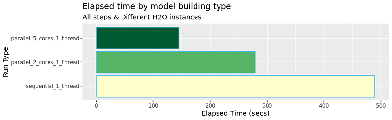
Iterations performed:

All steps & Different H2O instances
(each iteration loads the dataset and starts an H2O instance)

• Sequential (1 Thread for each iteration)
• Parallel (2 Cores — 1 Thread for each iteration)
• Parallel (5 Cores — 1 Thread for each iteration)

Optimized Steps & Unique H2O Instance
(the dataset it’s loaded once and only one instance it’s initiated)

• Grid (1 Thread for all iterations — parallelism level 1)
• Grid (2 Threads for all iterations — parallelism level 2)
• Grid (5 Threads for all iterations — parallelism level 5)
• Sequential (1 Core — 1 Thread for all iterations)
• Parallel (2 Cores — 2 Threads for all iterations)
• Parallel (5 Cores — 5 Threads for all iterations)

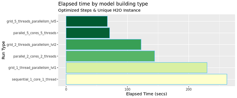
As expected, the H2O grid search is already quite optimized and it’s a very good solution. Although, and as mentioned, we can manage to implement more specific model creation processes with similar times, or even create a solution that brings together the best of both worlds: A parallel loop using H2O grid search to create several models. There is a big set of possibilities to make better use of our machine’s resources, speed up some analyses or even reduce costs in Azure and AWS services for example.

mclapply
Another way (more simple and direct) to enable parallel processing is to use the mclapply function from the parallel package. The mclapply function is basically a parallelized version of the lapply function.

The first two arguments to mclapply() are exactly the same as they are for lapply(). However, mclapply() has further arguments (that must be named), the most important of which is the mc.cores argument, that you can use to specify the number of processors/cores you want to split the computation across. For example, if your machine has 4 cores on it, you might specify mc.cores = 4 to break your parallelize your operation across 4 cores (although this may not be the best idea if you are running other operations in the background besides R)https://bookdown.org/rdpeng/rprogdatascience/parallel-computation.html

As an example to demonstrate mclapply, we will use the digit recognition dataset present in the Kaggle competition (https://www.kaggle.com/c/digit-recognizer).
In this demonstration we’ll transform the multinomial classification response (label:[0–9]) into several binomial classifications (isX: True or False), where, instead of creating a unique model to identify the ten digits, we are going to create 10 models (one model for each digit) with True or False probabilities. using the H2O AutoML functionality.
In this case, the division may not be the best solution, but in a scenario where you really need to create individual classification models based on the same knowledge data, the same data processing and modeling for different outputs, this can be a good and faster option.

library(parallel)
    library(data.table)
suppressPackageStartupMessages(library(h2o))
h2o.no_progress()

#Preparation
TRAIN <- read.csv("mnist_train.csv")
TRAIN <- as.data.table(TRAIN)
TEST <- read.csv("mnist_test.csv")
H2O_INIT_PORT <- 40000

predict_digit <- function(digit) {

# Init H2O (port from argument)
invisible(suppressWarnings(capture.output(
h2o.init(
port = H2O_INIT_PORT + digit * 3,
nthreads = 1,
max_mem_size = "1G"
)
)))

# Creating a personalized digit iteration train dataset with the appropriate response column
response <- paste0("is", digit)
it_train <- copy(TRAIN)
it_train <-
it_train[, eval(response) := ifelse(label == digit, TRUE, FALSE)]
it_train_hf <- as.h2o(it_train)
predictors <- setdiff(names(it_train), c(response, "label"))
it_test_hf <- as.h2o(TEST)

# Modelation - Auto ML
automl <- h2o.automl(
x = predictors,
y = response,
training_frame = it_train_hf,
nfolds = 5,
exclude_algos = c("GLM", "DeepLearning"),
balance_classes = TRUE,
max_runtime_secs = 300,
seed = 1234
  )

# Predict using automl leader model (best auc in xval)
prediction <- h2o.predict(automl@leader, it_test_hf)
prediction <- as.data.table(prediction)
names(prediction)[names(prediction) == "TRUE."] <- response

# Clear Iteration and shutdown h2o instance
h2o.removeAll()
h2o.shutdown(prompt = FALSE)

# returns the probability from being the iteration digit of every row from test dataset
return(prediction[, ..response])
}

We will use 10 cores, which means it will process an H2O AutoML for all digits at the same time. As you can notice in the script above, for each iteration, an H2O instance is initiated with 1 thread, each with its port. Each iteration will create as many models as possible in a maximum time of 300 seconds and then use the best model (automatically classified by H2O through the highest AUC value in cross-validation) to predict the labels of the test dataset.

system.time({
predictions <- mclapply(
X = 0:9,
FUN = predict_digit,
mc.preschedule = FALSE,
mc.cores = 10,
mc.cleanup = TRUE,
mc.silent = FALSE
)
})

predictions <- do.call(cbind, predictions)
predictions[, Label := colnames(.SD)[max.col(.SD, ties.method = "first")]]
predictions[, Label := gsub("is", "", Label)]

user | system | elapsed
87.369 | 9.970 | 408.359

The value shown for elapsed time is a good argument to confirm the advantage of carrying out a concurrent implementation for these types of cases. Had we not done so, the time would have been nine to ten times higher.

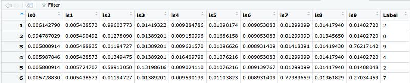
Not important for the demonstration, but the final result was a table with the probabilities of each row for each digit. With this table, you could build a final column with decisions supported from all models.

Final Remarks
And that’s it, a small demonstration, in many other possibilities, of the usage of concurrent processing in R with the H2O features. As demonstrated, H2O already provides a very effective way to build several machine learning models bypassing the limitations of R. If your purpose is to build a single model, selected for its performance, the grid search is a solid option and you may not need an extra R package to do it faster. But, if your problem requires building several different models, with similar data and preparation automatically built, evaluated and deployed, it is well worth the exploration and implementation of these parallel R packages. Based on the volume of data, you will have to choose between using a single instance in H2O with more resources or multi independent instances with fewer resources based on its pros and cons (time, jobs conflict, memory management, stability, …).
If the problem is even more complex, you can dockerize your solution and use Azure or AWS Batch services for example. The doAzureParallel package from Azure it’s very similar to doParallel, where we can distribute our processing to several machines at the same time. Perhaps a topic for an upcoming post!

References
https://cran.r-project.org/web/packages/doParallel/vignettes/gettingstartedParallel.pdf
https://privefl.github.io/blog/a-guide-to-parallelism-in-r/
https://bookdown.org/rdpeng/rprogdatascience/parallel-computation.html